Data

QuickStart Module

This quickstart module gives an overview of working with TimeSeries and Curve data.

TimeSeries

A TimeSeries is an array of values where each one is aligned to a point in time. Generally TimeSeries are used to record an event or observation at a particular timestamp. Example usage of TimeSeries:

• The price of a particular commodity
• The amount or volume of a product sold
• A computer hardware metric such as memory or CPU usage
• Some fundamental information such as the GDP or employment percentage of a country

Creating a TimeSeries

The minimum requirements for creating a TimeSeries is that it requires a Calendar. The calendar determines the intervals at which the observations will be recorded.

note

If the intervals are not pre-determined, you can use a Sparse calendar

Calendar

When constructing a TimeSeries using a calendar, you can either use the exact name of the calendar or a Calendar variable, e.g. in the following example ts1 and ts2 both use a Daily calendar

ts1 = TimeSeries("DAILY")
ts2 = TimeSeries(DailyCalendar())

Calendar, date and value

You can construct a TimeSeries with a calendar, a start date and a value or values e.g.

ts2 = TimeSeries("2021-10-01", "DAILY", 12.5)
ts3 = TimeSeries("2021-10-01", "BUSINESS", [12.5,12.6,12.7,12.8,12.9])

You can see that ts2 has been created with a single value of 12.5 for 1st October 2021.

We have created ts3 with 5 values starting at 1st October 2021 and because it is aligned to a BUSINESS calendar, the values skip the weekend, e.g.

[
2021-10-01  12.500000
2021-10-04  12.600000
2021-10-05  12.700000
2021-10-06  12.800000
2021-10-07  12.900000
]

The 2nd and 3rd of October are Saturday and Sunday, which are deemed as not-in-calendar days, so they are skipped.

Adding values

You add values to a TimeSeries using the built-in methods add or addValue.

Use add to tell the TimeSeries the date index of where to place the value and use addValue to place the value at the end of the TimeSeries at the next date index.

danger

When using add, the date index must align with the TimeSeries calendar, otherwise you will get an error.

ts3.add("2021-10-12", 14)
ts3.addValue(14.5)
print ts3.values

The output from that script shows:

[
2021-10-01  12.500000
2021-10-04  12.600000
2021-10-05  12.700000
2021-10-06  12.800000
2021-10-07  12.900000
2021-10-08  NaN
2021-10-11  NaN
2021-10-12  14
2021-10-13  14.500000
]

note

Note that we haven't added values for 2 date indexes, so these show as NaN or Not a Number

Saving TimeSeries

In order to save a TimeSeries, it needs to be added to an Object. You would usually create or use a specific type of object to store our TimeSeries on, but for simplicity we are just going to create a generic object.

QS01 = Object()
QS01.DATA = ts3

save ${object:QS01}

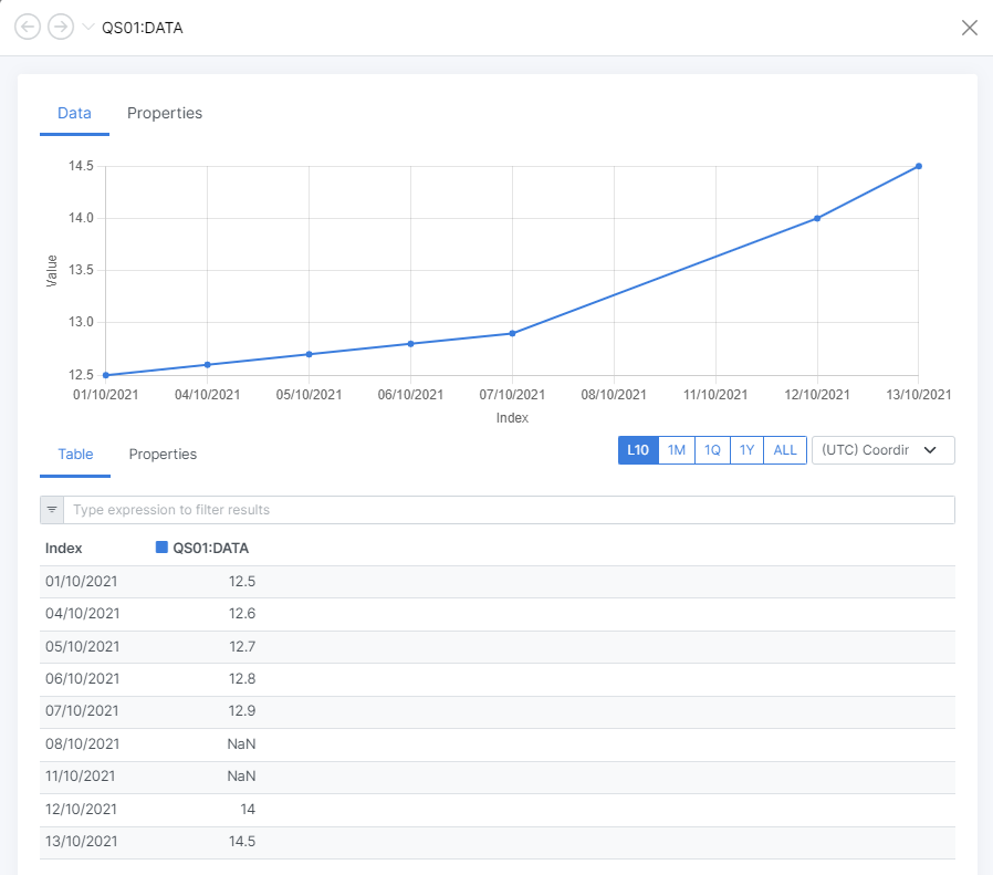
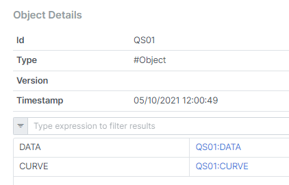
This will create an object called QS01 in our private repository and our TimeSeries will be called QS01:DATA. You can view both of these in the Web Portal as shown below:

Object explorer in the Web Portal

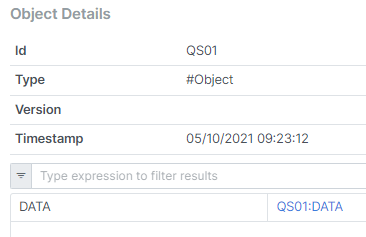
Data chart in the Web Portal

Updating TimeSeries

During the normal data collection process, we would be collecting values every day just updating that value to the TimeSeries. In OpenDataDSL, this is all handled for you, you simply create a mini-TimeSeries for the current value, update it and OpenDataDSL performs all the work required to blend the 2 TimeSeries.

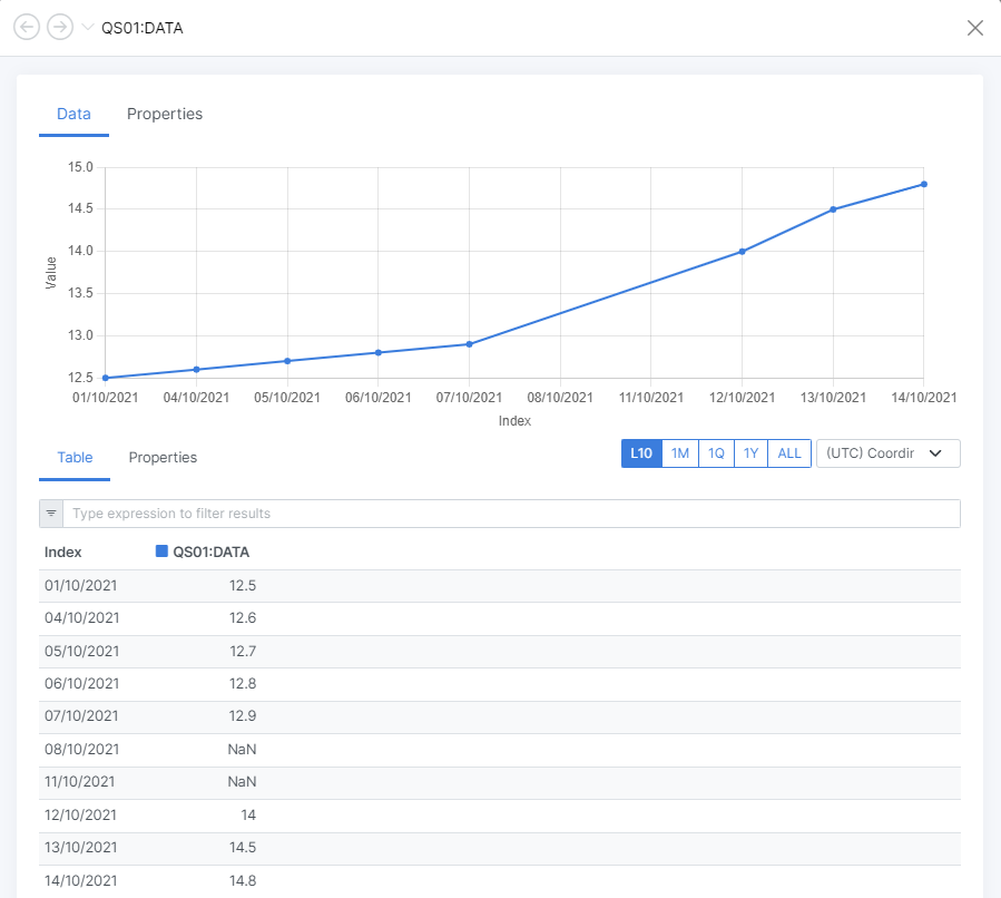
Take the following example of creating a single value for the 14th October 2021 and save it to QS01.

ts3 = TimeSeries("2021-10-14", "BUSINESS", 14.8)
QS01 = Object()
QS01.DATA = ts3
save ${object:QS01}

Reloading the data chart in the Web Portal shows the new value added

Data chart in the Web Portal

Changing TimeSeries Values

If configured, changing a TimeSeries value can trigger a new version of the TimeSeries to be written thereby preserving changes to all values. This is not covered in this QuickStart, but follow the link below to find out more.

In-Depth Information

TimeSeries Value Status

As well as values, you can also set a status per observation to record value metadata, such as:

• Quality
• Source
• Reliability

Example of setting the status of a value when adding it:

// Setting the status when the value is added
ts1 = TimeSeries("BUSINESS")
ts1.add("2021-10-15", 15.5, ["Valid", "Calculated"])

In-Depth Information

Curves

A Curve is a structure containing an array of contracts which each define a period of time in the future from the perspective of the curve. Example usage of Curves:

• Prices for the future delivery of a commodity, e.g. Oil or Wheat
• Forecast of power consumption for a country or region
• Weather forecasts

Creating a Curve

In order to create a curve, you need to create a CurveDate that defines the valuation or ondate of the curve.

The following code shows how to create a curve using a CurveDate of 1st October 2021 and an expiry calendar with the ID #REOMB.

// Create a valuation date
ondate = CurveDate("2021-10-01", "#REOMB")
// Create a curve
curve = Curve(ondate)

Adding Contracts

A Contract consists of a Period Code which defines the future referenced period and a value.

An example of adding a contract to our curve:

curve.add(Contract(ondate, "2021M11", 25.75))

This can be interpreted as: A price on 1st October 2021 of 25.75 for the delivery month November 2021

When a contract is created, a few calculations are performed about that contract, such as:

• The relative period code - M01
• The start of delivery - 2021-11-01
• The end of delivery - 2021-11-30
• The last trading date or expiry date - 2021-10-31

ondate = CurveDate("2021-10-01", "#REOMB")
c1 = Contract(ondate, "2021M11", 25.75)
print c1.relative
print c1.start
print c1.end
print c1.expiry

Saving a curve

Saving a curve is similar to saving a TimeSeries, we need to add it to an object and save the object.

We will use our existing object and add a curve to it, here is the code to do that:

QS01 = Object()
QS01.CURVE = curve
save ${object:QS01}

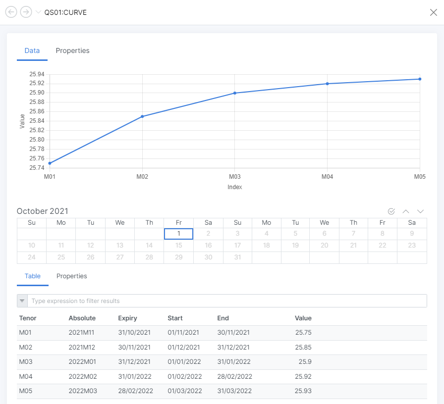
If you look at our QS01 Object in the Web Portal, you can now see that it has a CURVE added to it:

Object explorer in the Web Portal

We only have 1 contract added to the curve, so that chart only shows a single point, so let's add some more with the following code:

// Create a valuation date
ondate = CurveDate("2021-10-01", "#REOMB")
// Create a curve
curve = Curve(ondate)

curve.add(Contract(ondate, "2021M11", 25.75))
curve.add(Contract(ondate, "2021M12", 25.85))
curve.add(Contract(ondate, "2022M01", 25.90))
curve.add(Contract(ondate, "2022M02", 25.92))
curve.add(Contract(ondate, "2022M03", 25.93))
QS01 = Object()
QS01.CURVE = curve
save ${object:QS01}

A Curve differs from a TimeSeries in that you need to send the whole curve every time as it is a complete valuation. New curves for the same date are saved as a new version.

Curve in the Web Portal