Smart Curves
Introduction
Smart Curves are the easiest way of deriving new Forward Curves. They rely on having a real Forward Curve as a BASE in order to both determine when the curve has valuation dates and potentially to use in the Smart Curve expression.
In this tutorial, we show how to use Smart Curves writing ODSL code and using the REST API
Creating Basic Smart Curves
A Smart Curve can be created independently in ODSL code, but in order to save it to the database, you must add it to an Object.
The object can be a basic object or an object created from a Type
Using a basic object
A basic 'untyped' object is ok to use, but you maybe want to consider using either a public type or create your own private type.
In the example below, we are creating an object called CORN_TEST with a Smart Curve called CLOSE. The CLOSE curve is a backward filled CORN Forward Curve from MatbaRofex. We are also adding a 'category' property on the curve to easily filter and find it.
- OpenDataDSL
- REST API
// Creating using a basic object
CORN_TEST = Object()
CORN_TEST.CLOSE = SmartCurve("#MATBAROFEX.ROS.CORN.FUT:CLOSE", "bootstrapCurve(BASE)")
CORN_TEST.category = "TUTORIAL"

// Save to the database
save ${object: CORN_TEST}
POST https://api.opendatadsl.com/api/object/v1
Authorization: Bearer {{token}}

{
    "_id":"CORN_TEST",
    "_type":"#Object",
    "category": "TUTORIAL",
    "CLOSE":
    {
        "_id":"CLOSE",
        "_type":"VarSmartCurve",
        "baseCurve":"${data:'#MATBAROFEX.ROS.CORN.FUT:CLOSE'}",
        "expression":"interpolate(BASE, 'BACKWARD')"
    }
}
Creating using a type
This is the preferred method of creating objects, this categorises your objects correctly and implies a structure using default properties and dimensions of your object. You can read more about objects and types here.
- OpenDataDSL
- REST API
// Creating using a type
CORN_TEST_TYPE = object as #Agriculture
    CLOSE = SmartCurve("#MATBAROFEX.ROS.CORN.FUT:CLOSE", "interpolate(BASE, 'BACKWARD')")
    category = "TUTORIAL"
end

// Save to the database
save ${object: CORN_TEST_TYPE}
POST https://api.opendatadsl.com/api/object/v1
Authorization: Bearer {{token}}

{
    "_id":"CORN_TEST",
    "_type":"#Agriculture",
    "category": "TUTORIAL",
    "CLOSE":
    {
        "_id":"CLOSE",
        "_type":"VarSmartCurve",
        "baseCurve":"${data:'#MATBAROFEX.ROS.CORN.FUT:CLOSE'}",
        "expression":"interpolate(BASE, 'BACKWARD')"
    }
}
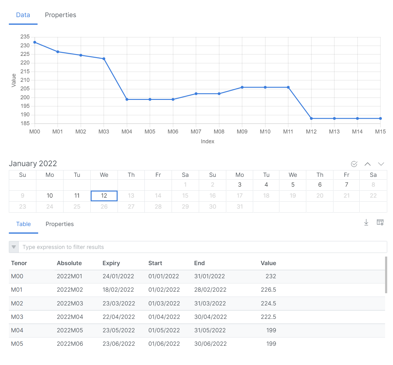
This is what the curve looks like when selected in the portal for a specific date:
Adding multiple Smart Curves to an object
You don't need to add a new object for every Smart Curve, you can add all related Smart Curves on the same object.
In this next example, we derive a premium curve from the CLOSE curve by adding a 15% increase in the prices.
This is achieved by using our CLOSE curve as the base curve and using an expression: BASE*1.15
- OpenDataDSL
- REST API
// Create a PREMIUM curve
CORN_TEST_TYPE = object as #Agriculture
    CURVE = SmartCurve("#MATBAROFEX.ROS.CORN.FUT:CLOSE", "interpolate(BASE, 'BACKWARD')")
    PREMIUM = SmartCurve("CORN_TEST_TYPE:CLOSE", "BASE*1.15")
    category = "TUTORIAL"
end

// Save to the database
save ${object: CORN_TEST_TYPE}
POST https://api.opendatadsl.com/api/object/v1
Authorization: Bearer {{token}}

{
    "_id":"CORN_TEST_TYPE",
    "_type":"#Agriculture",
    "category": "TUTORIAL",
    "CLOSE":
    {
        "_id":"CLOSE",
        "_type":"VarSmartCurve",
        "baseCurve":"${data:'#MATBAROFEX.ROS.CORN.FUT:CLOSE'}",
        "expression":"interpolate(BASE, 'BACKWARD')"
    },
    "PREMIUM":
    {
        "_id":"PREMIUM",
        "_type":"VarSmartCurve",
        "baseCurve":"${data:'CORN_TEST_TYPE:CLOSE'}",
        "expression":"BASE*1.15"
    }
}
Testing
If you are using ODSL to create the Smart Curves, you can also directly test the curve to see that it is creating the curve you expect before saving the Smart Curve to the database.
To test our CLOSE curve, we simply need to pick a date to test for and use the build method on the Smart Curve like shown below:
// Test our Smart Curve for 2022-01-12
CLOSE = SmartCurve("#MATBAROFEX.ROS.CORN.FUT:CLOSE", "interpolate(BASE, 'BACKWARD')")
print CLOSE.build("2022-01-12")
Smart Curves With Multiple Inputs
Not all curves derive from a single base curve, so you need to be able to reference other input data. For example, if you want to create a MID curve between a BID and OFFER, you need 2 curves in order to do this.
With Smart Curves, you can add references to other input data you require and then use them within the Smart Curve expression.
Multiple curve inputs
Using the MID example, we could use the BID curve as the Smart Curve base curve and add a reference to the OFFER curve, naming it OFFER. Your Smart Curve expression would then be:
(BASE+OFFER)/2
Here we see how to create this using the same MatbaRofex Corn curve, creating a MID between the MIN and MAX curves.
We are adding this Smart Curve to the object we created above
- OpenDataDSL
- REST API
// Add a MID curve to our existing Smart Curve
CORN_TEST_TYPE = ${object:"CORN_TEST_TYPE"}
CORN_TEST_TYPE.MID = SmartCurve("#MATBAROFEX.ROS.CORN.FUT:MIN", "(BASE+MAX)/2")

// Add a reference to the MAX curve
CORN_TEST_TYPE.MID.MAX = ref("data", "#MATBAROFEX.ROS.CORN.FUT:MAX")

// Save to the database
save ${object: CORN_TEST_TYPE}
POST https://api.opendatadsl.com/api/object/v1
Authorization: Bearer {{token}}

{
    "_id":"CORN_TEST_TYPE",
    "_type":"#Agriculture",
    "MID":
    {
        "_id":"PREMIUM",
        "_type":"VarSmartCurve",
        "baseCurve":"${data:'#MATBAROFEX.ROS.CORN.FUT:MIN'}",
        "expression":"BASE*1.15",
        "properties": {
            "MAX":"${data:'#MATBAROFEX.ROS.CORN.FUT:MAX'}"
        }
    }
}
Using scalar inputs
We can also add scalar values to the Smart Curve and use these within the Smart Curve expression.
In this example, we add a factor property to the Smart Curve and use it to scale the input curve.
- OpenDataDSL
- REST API
// Add a new curve using a factor
CORN_TEST_TYPE = ${object:"CORN_TEST_TYPE"}
CORN_TEST_TYPE.SCALED = SmartCurve("CORN_TEST_TYPE:CLOSE", "BASE*factor")

// Add the factor to the Smart Curve
CORN_TEST_TYPE.SCALED.factor = 0.8

// Save to the database
save ${object: CORN_TEST_TYPE}
POST https://api.opendatadsl.com/api/object/v1
Authorization: Bearer {{token}}

{
    "_id":"CORN_TEST_TYPE",
    "_type":"#Agriculture",
    "SCALED":
    {
        "_id":"SCALED",
        "_type":"VarSmartCurve",
        "baseCurve":"${data:'CORN_TEST_TYPE:CLOSE'}",
        "expression":"BASE*factor",
        "properties": {
            "factor":0.8
        }
    }
}
Using TimeSeries inputs
We may want to use values from a TimeSeries in our expression, for example if we want to apply a scaling factor which changes over time.
For this example we are going to create a Monthly TimeSeries on our object and populate it with 6 months of scaling factors which will be used to scale the CLOSE prices based on the month they are priced.
- OpenDataDSL
- REST API
// Use a TimeSeries scaling factor
CORN_TEST_TYPE = ${object:"CORN_TEST_TYPE"}

// Create a new TimeSeries with 6 months of scaling factors
CORN_TEST_TYPE.SCALER = TimeSeries("2022-01-01", MonthlyCalendar(), [0.82, 0.85, 0.86, 0.88, 0.9, 0.91])

// Create the Smart Curve
CORN_TEST_TYPE.TSSCALED = SmartCurve("CORN_TEST_TYPE:CLOSE", "BASE*SCALER")

// Add a reference to the Scaler TimeSeries
CORN_TEST_TYPE.TSSCALED.SCALER = ref("data", "CORN_TEST_TYPE:SCALER")

// Save to the database
save ${object: CORN_TEST_TYPE}
POST https://api.opendatadsl.com/api/object/v1
Authorization: Bearer {{token}}

{
    "_id":"CORN_TEST_TYPE",
    "_type":"#Agriculture",
    "TSSCALED":
    {
        "_id":"TSSCALED",
        "_type":"VarSmartCurve",
        "baseCurve":"${data:'CORN_TEST_TYPE:CLOSE'}",
        "expression":"BASE*SCALER",
        "properties": {
            "SCALER":"${data:'CORN_TEST_TYPE:SCALER'}"
        }
    },
    "SCALER":
    {
        "_id":"SCALER",
        "_type":"VarTimeSeries",
        "start":"2022-01-01",
        "calendar":"MONTHLY",
        "data":[
            {"time":"2022-01-01", "value":0.82},
            {"time":"2022-02-01", "value":0.85},
            {"time":"2022-03-01", "value":0.86},
            {"time":"2022-04-01", "value":0.88},
            {"time":"2022-05-01", "value":0.9},
            {"time":"2022-06-01", "value":0.91}
        ]
    }
}
Converting
You can specify a currency and units on Smart Curves and it will automatically convert all the input data to the chosen currency and units.
Converting currency
The curve that we have been using in the examples is in USD/MT, we can create a Smart Curve on our object in EUR/MT simply by specifying the currency and units of the Smart Curve.
- OpenDataDSL
- REST API
// Convert to EUR/MT
CORN_TEST_TYPE = ${object:"CORN_TEST_TYPE"}
CORN_TEST_TYPE.EUR_MT = SmartCurve("CORN_TEST_TYPE:CLOSE", "BASE")
CORN_TEST_TYPE.EUR_MT.currency = "EUR"
CORN_TEST_TYPE.EUR_MT.units = "MT"

// Save to the database
save ${object: CORN_TEST_TYPE}
POST https://api.opendatadsl.com/api/object/v1
Authorization: Bearer {{token}}

{
    "_id":"CORN_TEST_TYPE",
    "_type":"#Agriculture",
    "category": "TUTORIAL",
    "EUR_MT":
    {
        "_id":"EUR_MT",
        "_type":"VarSmartCurve",
        "baseCurve":"${data:'CORN_TEST_TYPE:CLOSE'}",
        "expression":"BASE",
        "currency":"EUR",
        "units":"MT"
    }
}
Converting units
Our corn units are Metric Tonnes (MT), so say instead we want to have a curve in USD per bushel (BU). According to researchgate.net the approximate density of corn is 721.
- OpenDataDSL
- REST API
// Convert to USD/BU
CORN_TEST_TYPE = ${object:"CORN_TEST_TYPE"}
CORN_TEST_TYPE.USD_BU = SmartCurve("CORN_TEST_TYPE:CLOSE", "BASE")
CORN_TEST_TYPE.USD_BU.currency = "USD"
CORN_TEST_TYPE.USD_BU.units = "BU"
CORN_TEST_TYPE.USD_BU.density = 721

// Save to the database
save ${object: CORN_TEST_TYPE}
POST https://api.opendatadsl.com/api/service/object/v1
Authorization: Bearer {{token}}

{
    "_id":"CORN_TEST_TYPE",
    "_type":"#Agriculture",
    "category": "TUTORIAL",
    "USD_BU":
    {
        "_id":"USD_BU",
        "_type":"VarSmartCurve",
        "baseCurve":"${data:'CORN_TEST_TYPE:CLOSE'}",
        "expression":"BASE",
        "currency":"USD",
        "units":"BU",
        "properties": {
            "density":721
        }
    }
}
Custom Algorithms
In order to create a curve exactly how you want it, there are occasions where you would need to create your own algorithms. The custom code you write will be ODSL code and usually you would create a user definable function in a script. The Smart Curve expression would then call your custom function.
Creating a custom script
The easiest way to create an ODSL script is to use the VS Code extension.
In our example, we are going to create a function that creates a time spread curve which calculates the spread between the tenors of an input curve.
-
Create a file called
MyFunctions.odsl -
Paste this code into the file
function timespread(input)
    // Create a curve with spreads created from the months in the input curve after bootstrapping
    boots = bootstrapCurve(input)
    timespread = Curve(input.ondate)
    last = boots.contracts[0]
    for i = 1 to boots.contracts.size - 1
        m = boots.contracts[i]
        value = m.value - last.value
        spread = Contract(input.ondate, last.tenor + "-" + m.tenor, value)
        timespread.add(spread)
        last = m
    next
end
- Save the file to the DataBase by right-clicking in the editor and select
Upload this script
Testing our code
We can insert some code above our function to run a simple test to make sure the function is producing the correct results.
Paste the following code above the function in the script and run it.
ondate = CurveDate(Date("2022-01-12"), "#REOMB")
curve = Curve(ondate)

curve.add(Contract(ondate, "2022M02", 25.67))
curve.add(Contract(ondate, "2022M03", 25.75))
curve.add(Contract(ondate, "2022M04", 26.75))

ts = timespread(curve)
print ts
This produces the following output which shows a time spread curve from the simple input curve:
id: ts
date: 2022-01-12
ccy/units: null/null
==== Contracts ====
M01-M02: 0.080000
M02-M03: 1.000000
==== Properties ====
{}
Creating a Smart Curve to use the script
As previously, we need to add a Smart Curve onto our object to use our custom script. We add the name of the script onto the Smart Curve, so it knows to use our script rather than the default Smart Curve script.
// Using a custom script
CORN_TEST_TYPE = ${object:"CORN_TEST_TYPE"}
CORN_TEST_TYPE.TIMESPREAD = SmartCurve("CORN_TEST_TYPE:CLOSE", "timespread(BASE)")
CORN_TEST_TYPE.TIMESPREAD.script = "MyFunctions"

// Save to the database
save ${object: CORN_TEST_TYPE}
A function that calls the standard functions
If you want to use the Smart Curve functions in your custom function, you will need to import the standard functions in your custom function script.
This is achieved by adding the following line at the top of your script:
import ${script:"#CurveScript"}